Why Forecasters are Fixated with Accuracy — The Risk of Ignoring Feedback

By Claudio Antonini and Kamil Mizgier

In discussions about forecasting it might serve well to remember its mothership: the field of control theory. In this field, the objective is to control a system, sometimes called a ‘plant’ which, for example, can be a robotic arm, a submarine depth system, or an interplanetary probe telescope camera. To control these systems, actions must be implemented and, conceptually, they can be grouped in two processes that work in unison: one process commands the plant and another process estimates the variables on which the control is based. Let us consider an airplane: if the objective is to maintain course at a certain speed and altitude, the control part would be exercised by the combined actions of a turbine and a few control surfaces (ailerons, rudder), and the variables to be estimated will be the airspeed, attitude, and altitude, among others. In an economic system, the commands may be taxation, interest rates, or import restrictions and the estimates may be the level of employment, inflation rate or currency exchange.

Whatever the specific variables controlled or estimated, overall, the fundamental and critical feature that allows a system to follow commands–to be controlled–is feedback. This mode of working, when feedback is implemented, is called “closed-loop.” Conversely, without feedback, the system would be labelled “open-loop.” Summarizing, no feedback, no control.

Compared to open-loop systems, feedback helps in (a) reducing the effect of modelling error and external disturbances, (b) changing–if necessary–the whole system stability, and (c) improving accuracy, that is, the ‘distance’ to a desired setpoint. In the case of an airplane, if feedback is broken for some reason, the airplane would not be able to use the estimated (also called, forecasted) variables and would not be able to be controlled. Effectively, the airplane would be unable to maintain its required speed and altitude. The nightmare of a control engineer is an open-loop, uncontrolled system.

The arrangement of dividing control in two processes–control itself and estimation (depending on the author and disciplines also known as ‘filtering’ or ‘forecasting’) –is well illustrated in a seminal book, “Time Series Analysis: Forecasting and Control,” by George Box and Gwilym Jenkins¹. A testament to the importance of the book is that it has seen five editions since its first, in 1970. In this work, Box and Jenkins consider time- and frequency-domain techniques to analyze systems described by their time-series, stressing time and again that the most important characteristic of a control system is its stability. However, nowadays, Box and Jenkins is rarely, if ever, quoted in forecasting literature. Forecasters are focused on other performance parameters of the system and may not be aware of the possibility of controlling it to get even better performance.

Most likely, practitioners ignore feedback due to their restricted focus, not paying attention to topics that Box & Jenkins discussed over various editions of their book. Forecasters today apply techniques almost exclusively in the time domain (except for some work with FFTs); do not consider transfer functions; have not heard of poles or zeros; and do not have ways of measuring the system’s stability. Effectively, forecasting is working in an open-loop architecture and, for that reason, practitioners are so concerned with ‘accuracy,’ something that, in a closed-loop system, is of secondary concern when compared to the primary importance in that field: stability.

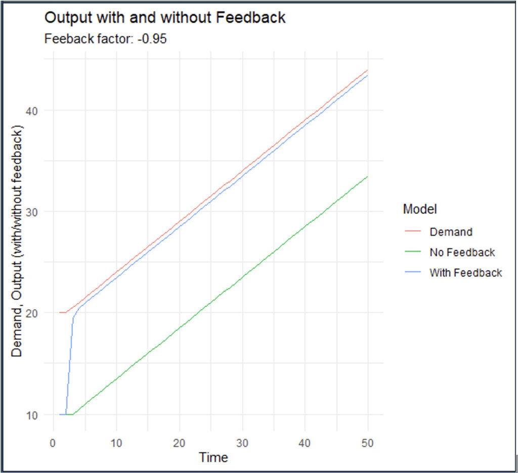
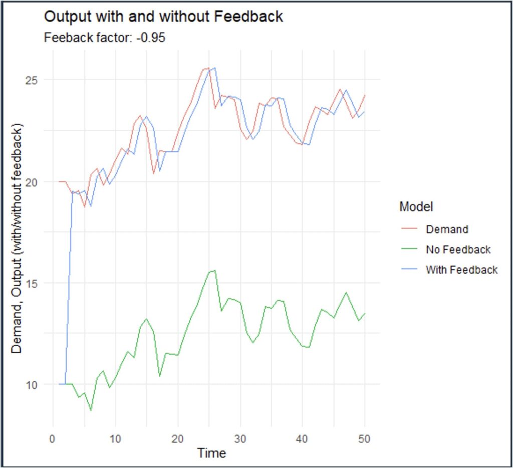
Several studies have been published that aim to model closed-loop systems, particularly in areas such as economics² and supply chain management³. We illustrate this concept by running a small program to simulate supply and demand for a hypothetical demand-planning exercise. In this model, we simulate the output (or quantity produced) based on demand and observe how closing the feedback loop affects the accuracy of our predictions. In the first model run, the simulation assumes that demand grows linearly. In the second run, we enhance the model by introducing randomness to demand. The no-feedback model simply uses the demand from the previous two samples to predict how it will grow in the next sample. The formula is as follows

which is a very simple linear demand forecasting model.

In comparison, the feedback model adjusts predictions by applying a correction factor based on how far the actual output (output_with_feedback) deviated from the demand in the previous sample (demand[t-1]), effectively closing the loop. In formula

The results of the simulations with feedback and without it are shown below in Figure 1 (demand grows linearly) and Figure 2 (random demand).

Figure 1. Production output with and without feedback (linear demand).

Figure 2. Production output with and without feedback (random demand).

In both cases, we see a solid improvement in terms of accuracy (getting closer to the demand) even when that was not a design objective.

The large improvement in accuracy is attributed to using a new structure for minimizing the error. This is a profound difference with articles that analyze alternative methods to improve accuracy where different methods for forecasting are employed but always keeping the same open-loop structure. In this case, we are closing the loop, departing significantly from minimal changes in algorithms that keep the same open-loop structure.

But … why do forecasters ignore feedback?

Most probably, forecasting practitioners deal with types of systems in which they cannot model the feedback process and, thus, “what one cannot model one cannot control.” These are possible reasons:

• social systems are more difficult to model than physical systems which follow well-known laws
• events in social systems are single-case experiments – rarely they can be repeated
• even if they were successfully modeled, humans would try to exploit loopholes and react in ways that were not considered during the modeling phase (the Lucas’ principle in economics)
• believing that forecasting demand (although useful in itself) is a substitute (in terms of performance) to having a model for the feedback process.

In addition to the fuzziness of the social systems that forecasters must deal with, in social environments the time scales are orders of magnitude slower than those in physical systems. In the case of an airplane’s autopilot, typically, the signals that are used to estimate aileron or rudder positions and turbine parameters are sampled every few milliseconds. Thus, humans may not be able to control the airplane in real-time (particularly naturally unstable airframes) and the control has to be automated. On the other hand, forecasting sales in a supermarket may have to be done with monthly data, or macroeconomic systems with quarterly data. That data in these cases is available so infrequently may give the idea to humans that they have ample time to make decisions and affect outcomes of their system (sales, output in a GDP, unemployment …) in a desired direction. To that effect they indeed take action, but without the rigor of a control engineer, who makes a significant effort in modeling the system to be controlled, and simulating various techniques to get desired outcomes.

Either because of choice (relying on modeling demand and ignoring modeling the feedback decision process), necessity (social systems difficult to model or data available too infrequently), or lack of familiarity with modeling techniques (relying on crude and simple regressions instead of more dynamic approaches), and confronted with systems that behave under their own open-loop dynamics, forecasters have no other possibility than measuring how far they are from an intended target. That is, they have no other possibility than to keep developing and using ‘accuracy’ indicators, much like a man walking on the middle of the street decides that it does well if he hits the curb in 3 minutes of walking blind instead of 1 minute.

Comparing feedback and no-feedback prediction models, it becomes evident that human-controlled systems often fail to achieve optimal performance, as compared to airplanes and other engineered systems. Systems overwhelmed by exploding amount of information and indicators can exacerbate problems rather than resolve them. Such control relies heavily on noisy, incomplete, or misleading data, which can result in decisions that decrease performance.

The key takeaway is that resilience should be a design concern in case of performance degradation. Systems that prioritize adaptability and robustness—while acknowledging the limits of prediction—are better equipped to deal with uncertainty and mitigate risks. For example, flood prediction systems in Europe have failed multiple times in 2024, highlighting the dangers of relying too heavily on inaccurate weather forecasts without building sufficient resilience into the system. Needless to say, in cases where feedback modeling could be implemented, ignoring it would be a risky–if not negligent–endeavor.

About the Authors

Dr. Claudio Antonini, MIT nuclear safety engineer, after working in the design of GNC systems for missiles and drones, has applied that numerical experience in the field of finance for the last 25 years. Working at UBS, developed the largest global implementation of a genetic algorithm for banking, and has continued to apply data mining, machine learning, and artificial intelligence algorithms for risk management, in consultancies (Deloitte, AlixPartners) and the Bank of New York Mellon. He publishes consistently on forecasting topics.

Dr. Kamil Mizgier brings his extensive practical experience and deep knowledge to explore challenges in strategic risk management. By leveraging his 15 years of expertise from key roles, including Global Supplier Relationship and Risk Management Leader at Dow and risk modeling leadership positions at BNY Mellon and UBS, he delves into the latest trends, tools, and techniques in risk management, offering invaluable perspectives that bridge academic rigor and practical application.

References

1. Box, G. et al. 2015. “Time Series Analysis: Forecasting and Control.” 5th Edition, John Wiley and Sons Inc., Hoboken, New Jersey.

2. Carranza, R. G. 2016. ”The Closed Loop Economy.” International Journal of Design & Nature and Ecodynamics, 11(4), pp. 600-609.

3. MahmoumGonbadi, A. et al. 2021. “Closed-loop supply chain design for the transition towards a circular economy: A systematic literature review of methods, applications and current gaps.” Journal of Cleaner Production 323 : 129101.